Basic Optimizations with H2MM_C#
See also
This can also be viewed as a Jupyter Notebook
Download H2MM_Optimization_Tutorial-OOP.ipynb
The data files can be downloaded here: sample_data_2det.txt sample_data_3det.txt
First let’s import some standard modules:
import os
import numpy as np
from matplotlib import pyplot as plt

import H2MM_C as hm
Basic Analysis#
The base steps of analysis with H2MM are:
Load data
Make initial model
Optimize model
Viterbi analysis to classify photons and assess quality of optimization
Note
Steps 2-4 are usually repeated multiple times with different numbers of states and result compared to select the ideal model
Step 1: Load Data#
Now that the data is imported, we can start to perform the basic analysis of H2MM, for which we will need some data to analyze. So we will load some data with the following lines of code:
# This cell will only be used if you export your data to an ascii file,
# if you are using a software package such as FRETBursts, a different
# function (for FRETBursts, look at our other Jupyter Notebooks, it is
# the data_sort function)
def load_txtdata(filename):
    color = list()
    times = list()
    with open(filename,'r') as f:
        for i, line in enumerate(f):
            if i % 2 == 0:
                times.append(np.array([int(x) for x in line.split()],dtype=np.int64))
            else:
                color.append(np.array([int(x) for x in line.split()],dtype=np.uint8))
    return color, times

color2, times2 = load_txtdata('sample_data_2det.txt')
Data Organization#
So what does this data look like? It comes in 2 lists of arrays. One list contains the detectors (indices) of the data. The second, the times of the data.
color2 contains the detectors
times2 contains the times of the data
Both are lists of 1-D numpy arrays.
Note
The size of the detector list and time list, and of the arrays within must match. This is because each data point is a pair of numbers: the index of the detector, and the absolute time of the data point. Each array (element of the two lists) is a sequence of data that is to be analyzed as a separate instance of data that can be represented by the same hidden Markov model. Therefore the length of color2 must be the same as the length of times2 Similarly, the length of the first array in color2 must be the same as the length of the first array in times2. The lengths of the second arrays in color2 and times2 must also match, and so on. There is no need however for the lengths of the first and second arrays in color2 and times2 to match, as sequences of data points need not be the same length.
For the next step, it is important that the number of detectors is known, as this affects the initial model to be used. In the example loaded above, there are 2 detectors- 0 and 1.
Note
Indices must start from 0 and go in integer ascending order. I.E. if there are 2 detectors, you must use indices 0 and 1. Similarly, if there are 3 indices you must use indices 0, 1 and 2. And so on.
>>> color2[0], times2[0]
(array([1, 0, 1, 1, 0, 0, 0, 0, 1, 0, 0, 1, 1, 0, 0, 0, 0, 0, 0, 1, 1, 1,
        1, 1, 1, 1, 0, 1, 1, 0, 0, 1, 0, 0, 1, 1, 1, 1, 1, 0, 0],
       dtype=uint64),
array([12763662, 12766593, 12769260, 12769677, 12775221, 12781399,
        12783890, 12795124, 12795391, 12796727, 12797800, 12798471,
        12798527, 12799163, 12799626, 12802748, 12808470, 12811473,
        12826887, 12841103, 12842716, 12842791, 12844203, 12844446,
        12845687, 12846645, 12847506, 12848115, 12850099, 12853216,
        12853259, 12853526, 12853632, 12853845, 12855027, 12858436,
        12858750, 12860935, 12861560, 12861894, 12869843], dtype=uint64))
Step 2: Create an Initial Model#
H2MM is fundamentally an optimization, which means that an initial, unoptimized model must be used as a starting point to initiate the optimization.
These models are represented by the h2mm_model in H2MM_C
H2MM_C provides a simple function for creating initial models: factory_h2mm_model().
All you need to do is specify the number of states and the number of detectors.
Note
The number of states is arbitrary, as we will show later. You should compare several different numbers of states. The number of detectors, however is determined by your data. For the file sample_data_2det.txt there are 2 detectors.
So let’s make the initial model. The syntax is: hm.factory_h2mm_model(nstate: int, ndet: int):
So let’s make an initial model:
model_3s2d = hm.facotry_h2mm_model(3,2) # 3 states, 2 detectors
Step 3: Optimize the Model#
Now that we have an initial model, we can optimize it against the data.
For this we use the h2mm_model.optimize() method.
The syntax is
model.optimize(indexes: list[numpy.ndarray], times: list[numpy.ndarray])
So let’s optimize the model:
model_3s2d.optimize(color2, times2)
model_3s2d
Examining the optimized model#
The core of a h2mm_model is composed of 3 arrays.
In the following definition, N will indicate the number of states, and M the number of detectors.
h2mm_model.prior: the initial probability vector, of shape N, which represents the probability of a sequence beginning in each state.h2mm_model.trans: the transition probability matrix, of shape N by N, the probability of a transition happenign from state i to state j. .. note:The units of the transition probability matrix are in units of the clock-rate of the data
h2mm_model.obs: the emission probability matrix, of shame N by M. The probability that if the system is in state i, the detector j will be observed.
Note
All the above arrays are row stochastic meaning that the sum of the values in each row sum to 1. This is because these are all probabilities and each row enumerates all possibilities, thus their total probability must be 1. Calculate values accordingly
These are all printed as part of the reper for h2mm_model
There are a number of other secondary parameters stored in the h2mm_model object.
The size of the matricies can be accessed with
h2mm_model.nstatethe number of statesh2mm_model.ndetthe number of detectors
Others are specific to the course of the optimization
h2mm_model.niterThe number of iterations during the optimizationh2mm_model.nphotThe number of data points in the input data on which the model was optimized
There are the statistical parameters that reflect the likelihood of the model:
h2mm_model.loglikThe loglikelihood of the model. This represents the value which is being optimized.h2mm_model.bicThe Bayes Information Criterion, a statistical discriminator. \(BIC = k\ln(n) - 2\ln(LL)\) where \(k = nstate^2 - (ndet - 1)nstate - 1\), this is used for comparing loglikelihoods of different models with different numbers of states, but optimized against the same data.h2mm_modle.kThe number of free parameters in the model.
Step 4: Viterbi Analysis#
The final step in the H2MM analysis of a single model is to find the most likely state-path through the data. This is done using the Viterbi algorithm.
For this H2MM_C has the viterbi_path() function.
This function returns the most likely state path as well as a few other useful values.
These values are:
path: The most likely state of each data pointscale: the likelihood of each state assignment inpath, i.e. the posterior probabilityloglik: The loglikelihood of each trajectory, returned as a numpy array.ICL: The Integrated Complete Likelihood, a statistical discriminator, which is essentially the \(BIC\), but for the most likely path instead of all possible paths.
The syntax is:
hm.viterbi_path(model: H2MM_C.h2mm_model, indexes: list[numpy.ndarray], times: list[numpy.ndarray])
path_3s2d, ll_3s2d, icl_3s2d = hm.viterbi_path(model_3s3d, color2, times2)
path_3s2d[0]
Loop Based Analysis#
Since we need to compare different models, it is generally more usefull to run the analysis in a loop, and then compare the different optimizations.
In particular, the ICL is very useful in identifying the best model.
We will also now use a data set with 3 detectors, so that we can see how different detector numbers affect the analysis code.
# load the data
color3 = list()
times3 = list()

i = 0
with open('sample_data_3det.txt','r') as f:
    for line in f:
        if i % 2 == 0:
            times3.append(np.array([int(x) for x in line.split()],dtype='Q'))
        else:
            color3.append(np.array([int(x) for x in line.split()],dtype='L'))
        i += 1
For this we will start with a simple loop, optimizing for 1 to 4 states (there’s no such thing as a 0 state model)
# initiate lists
models = list()
paths = list()
scales = list()
logliks = list()
ICL = list()

# loop from 1 to 4 states
for i in range(1,5):
    # make initial model with i states
    model_temp = hm.factory_h2mm_model(i, 3) # i states, 3 detectors
    # optimize model
    model_temp.optimize(color3, times3)
    # calculate ideal state path
    path_temp, scale_temp, ll_temp, icl = hm.viterbi_path(model_temp, color3, times3)
    # append results to lists
    models.append(model_temp)
    paths.append(path_temp)
    scales.append(scale_temp)
    logliks.append(ll_temp)
    ICL.append(icl)
models
Now that several models have been calculated, it is important to select the ideal model, so you do not use over- or under-fit models that do not properly represent the data.
There are two primary criterion for this:
A statistical discriminator like the ICL or BIC
Reasonableness of the model based on prior knowledge of the system.
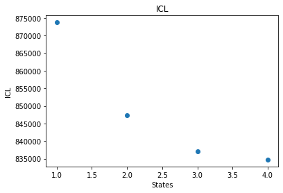
So let’s plot the ICL to see what the best model is:
states = np.arange(1,5)
plt.scatter(states, ICL)
plt.xlabel("States")
plt.ylabel("ICL")
plt.title("ICL")
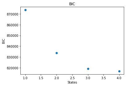
states = np.arange(1,5)
plt.scatter(states, [model.bic for model in models])
plt.xlabel("States")
plt.ylabel("BIC")
plt.title("BIC")
So it looks like the ideal model (minimum ICL) is the 4 state model.
But since this is also the most number of states optimized, a 5 state model might be even better. Even if the 4 state model is best, seeing that the ICL of the 5 state model increases, it is still best to optimize it so that we can be assured that the 4 state model is best. And if the 5 state model turns out to have an even smaller ICL, we should go on and optimize a 6 state model.
model_temp = hm.factory_h2mm_model(5,3)
model_temp.optimize(color3, times3)
path_temp, scale_temp, ll_temp, icl = hm.viterbi_path(model_temp, color3, times3)
models.append(model_temp)
paths.append(path_temp)
scales.append(scale_temp)
logliks.append(ll_temp)
ICL.append(icl)
states = [model.nstate for model in models]
bic = [model.bic for model in models]

fig, ax = plt.subplots(1,2, figsize=(12,5))

ax[0].scatter(states, ICL)
ax[0].set_xlabel("States")
ax[0].set_ylabel("ICL")
ax[0].set_title("ICL")

ax[1].scatter(states, bic)
ax[1].set_xlabel("States")
ax[1].set_ylabel("BIC")
ax[1].set_title("BIC")
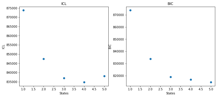
Indeed, it looks like the 4 state model is the ideal model, so let’s examine it:
models[3]
User Defined Initial Models#
Usually the factory_h2mm_model() function is sufficient for generating initial models, however, sometimes it is preferable to define the parameters of the initial model more manually.
This is done like so:
# define input prior, trans and obs matrices
prior = np.array([0.5,0.5])
trans = np.array([[0.99999, 0.00001], [0.00001, 0.99999]])
obs = np.array([[0.2, 0.3, 0.5], [0.4, 0.2, 0.4]])

# make the initial model
model_user = hm.h2mm_model(prior, trans, obs)
We can optimize this just as before:
model_user.optimize(color3, times3)
model_user
h2mm_model.evaluate() and Error Analysis#
See also
H2MM_arr() and Error Analysis which uses the H2MM_arr() instead.
While in most other cases there is no practical difference in using the functional vs object oriented apprach, here, h2mm_model.evaluate() will be slower, because there is more python interaction.
This is because some pre-processing must be done on the input data, which will be done every time h2mm_model.evaluate() is called, while if used appropriately H2MM_arr() will only do this once, and even features a few C level optimizations for iterating through the models, all this is lost when using the object oriented approach.
You will notice that so far H2MM analysis has not given any estimation of the error of the parameter values.
One way to estimate the error is to compare how quickly the loglikelihood falls off as a given parameter is varied around the optimized value.
For this we not to just evaluate the loglikelihood of a model, instead of optimizing the model (we already have the optimized model).
To merely evaluate the loglikelihood of a model against some data, we have the h2mm_model.evaluate() function.
The method call is identical to h2mm_model.optimize():
hm.H2MM_arr(models: list[hm.h2mm_model], indexes: list[numpy.ndarray], times: list[numpy.ndarray])
For error evaluation, we will make a list of models, and vary just one value in them. Since the 4 state model looks like the best model, lets try this on that model, and change the most interesting transition rate, that from state 1 to state 2 (states indexing from 0 since this is python after all).
# pull out the parameters of the model
prior_4s3d = models[3].prior
trans_4s3d = models[3].trans
obs_4s3d = models[3].obs

error_models = list()
for tk in np.linspace(-2e-6, 2e-6, 41):
    new_trans = trans_4s3d.copy() # copy so that tweeks can be make without changing the original array
    new_trans[1,2] += tk
    new_trans[1,1] -= tk # adjust the diagonal so that matrix remains row stochastic
    tk_model = hm.h2mm_model(prior_4s3d, new_trans, obs_4s3d)
    tk_model.evaluate(color3, times3)
    error_models.append(tk_model)
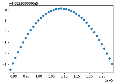
Now we can plot the loglikelihood and see how sharply it is centered on the optimal model:
trs  = [model.trans[1,2] for model in error_models]
ll = [model.loglik for model in error_models]

plt.scatter(trs, ll)
plt.xlim([min(trs)-5e-8, max(trs)+5e-8])